Last week I uploaded a note about the paper @freakonometrics and I have submitted again after we added quite a few revisions. We have already made available most of the R code to reproduce our applications (on this GitHub repository). However, we did not share our method to obtain the coordinates of the « hot-spots » areas, as those visible on the following map:
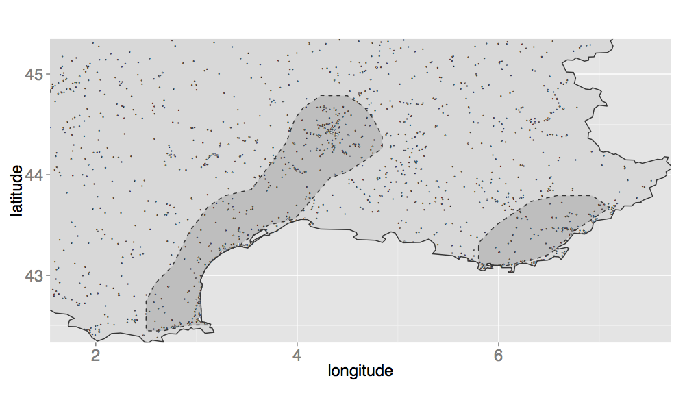
The hot-spots areas are obtained using the values of the density estimates. Those estimates are computed at some locations, and we use a function called « geom_tile() » to represent them on a map. It is easy to visualize the hot-spots area on a map, but it gets a bit complicated to create a polygon out of these points. There is an interesting function in the package alphahull, namely ashape(), which calculates the alpha-shape of a sample. When calling the plot.ashape() function, it is possible to visually identify multiple areas. But when we looked at the code of the plot.ashape() function, we were a bit disappointed to see that there is actually no polygon defined. Instead, a series of segments are drawn, and not necessarily in a convenient order! Besides, these segments are not intersecting…
So, we decided to use the result from ashape() to try and extract the coordinates of any area. Our technique requires some handiwork. The basic idea here is that we rely on some statistical classification based on the distance separating each points. We need to create more clusters than the number of areas we desire, and then we manually regroup some clusters (by clicking on a graph).
The rest of this note is divided as follows: a section introducing the functions, then a first example, and a second one.
A fun application can be seen on @freakonometrics‘ blog.
Let’s roll!
Functions
First, we need to load some packages:
library(ellipse)
library(fields)
library(gpclib)
library(ks)
library(maps)
library(rgeos)
library(snow)
library(sp)
library(ggmap)
library(reshape2)
library(alphahull)
library(fossil)
library(geosphere)
Now, we need a few functions.
The function get_coords_pol() returns the indices of points in a given polygon (`polygon`) that define a convex hull. The result of this function is useful for the next function, coords_pol().
# @polygon:  data.frame containing coordinates of points inside a hull
# @alpha:    alpha value
get_coords_pol <- function(polygon, alpha = .25){
  alpha_shape <- ashape(polygon, alpha = alpha)
  id <- alpha_shape$edges[, 1:2]
  loop <- FALSE
  listi <- id[1,1:2]
  vk <- 2:nrow(id)
  i0 <- as.numeric(listi[length(listi)])
  while(!loop){
    idxi0 <- which(id[vk,1] == i0)
    if(length(idxi0) > 0) {nb <- id[vk,2][idxi0]}
    if(length(idxi0) == 0) {
      idxi0 <- which(id[vk,2]==i0)
      nb <- id[vk,1][idxi0]
    }
    if(length(idxi0) == 0) {loop <- TRUE}
    if(!loop){
      listi <- c(listi,nb)
      vk <- vk[-idxi0]
      i0 <- nb
    }
  }
  res <- listi
  names(res) <- NULL
  res
}# End of get_coords_pol()
The function coords_pol() returns a `data.frame` containing the coordinates of a polygon defining a convex hull, according to a cluster ID (clust).
# @clust:     cluster id
# @polygons:  data.frame containing coordinates of each points
#             and cluster associated (as returned by pre_cut_help())
coords_pol <- function(clust, polygons, pol, ...){
  ind <- which(polygons[, "clust"] == clust)
  polygon <- unique(polygons[ind, c("x2", "y2")])
  coords_ind <- get_coords_pol(polygon, ...)

  res <- polygon[coords_ind,]
  colnames(res) <- c("long", "lat")

  # Intersection avec le polygon
  coords_pol_inter <- intersect(as(res, "gpc.poly"), pol)
  df_res <- data.frame()
  for(i in seq_len(length(coords_pol_inter@pts))){
    df_tmp <- data.frame(long = coords_pol_inter@pts[[i]]$x,
                         lat = coords_pol_inter@pts[[i]]$y,
                         hole = coords_pol_inter@pts[[i]]$hole,
                         group = i)
    df_res <- rbind(df_res, df_tmp)
  }
  df_res
}# End of coords_pol()
The function pre_cut_help() returns a data.frame where each point corresponds to a point from the density estimation where the value is above the decided threshold. Each point is associated to a possible polygon. The data.frame that is returned can be viewed as a preliminary cutting. This function is then used in pre_cut_f().
# @alphashape:  alpha-shape list returned by ashape()
# @k:           number of desired groups
pre_cut_help <- function(alphashape, k){

  # Edges
  alphashape_df <- data.frame(alphashape$edges)
  alphashape_df <- alphashape_df[, c("x1", "y1", "x2", "y2")]

  to_remove <- which(duplicated(alphashape_df[, c("x1", "y1")]))
  alphashape_df <- alphashape_df[-to_remove,]
  rownames(alphashape_df) <- NULL
  alphashape_df$id <- seq_len(nrow(alphashape_df))

  distance_deg <-  function(long1, lat1, long2, lat2) {
    R <- 6371
    acos(sin(lat1)*sin(lat2) + cos(lat1)*cos(lat2) * cos(long2-long1)) * R
  }# End of distance_deg()

  # http://stackoverflow.com/questions/21095643/approaches-for-spatial-geodesic-latitude-longitude-clustering-in-r-with-geodesic
  geo.dist = function(df) {
    d <- function(i,z){# z[1:2] contain long, lat
      dist <- rep(0,nrow(z))
      dist[i:nrow(z)] <- distHaversine(z[i:nrow(z),1:2],z[i,1:2])
      return(dist)
    }
    dm <- do.call(cbind,lapply(1:nrow(df),d,df))
    return(as.dist(dm))
  }
  hc <- hclust(geo.dist(alphashape_df[, c("x2", "y2")]))
  alphashape_df$clust <- cutree(hc, k = k)

  alphashape_df
}# End of pre_cut_help()
The function pre_cut_f() returns a preliminary cutting of the different areas where the density estimates are above a threshold. This is the starting point of the method used to obtain coordinates of convex hulls. The result is a list of two elements :
pre_cut_df: adata.framecontaining information about each density estimate above the threshold, including the ID of the polygon in which it lies;pre_cut_polys: a list whose elements aredata.frameobjects, containing coordinates of every polygon defined./li>
# @x:         density estimates as returned by sKDE()
# @threshold: threshold to use
# @alpha:     value of alpha in the alpha-shape hull calculation (ashape())
# @poly:      bounding polygon, as a data.frame, where first column must be longitude
#             and second column latitude coordinates
# @k:         number of desired groups
# @print:     if FALSE, does not plot the result
pre_cut_f <- function(x, threshold, alpha, poly, k, print = TRUE){

  # Extract points where density estimates are greater or equal to the threshold
  pts_sup_ind <- which(x$ZNA >= threshold, arr.ind = TRUE)
  pts_sup <- data.frame(long = x$X[pts_sup_ind[,1]],
                        lat = x$Y[pts_sup_ind[,2]])

  pts_sup <- pts_sup + rnorm(sum(x$ZNA >= threshold, na.rm = TRUE)*2)/1000

  # alpha-shape hull calculation
  alphashape <- ashape(pts_sup, alpha = alpha)


  pre_cut_df <- pre_cut_help(alphashape, k = k)

  pre_cut_polys <- lapply(unique(pre_cut_df$clust), coords_pol,
                            polygons = pre_cut_df, pol = as(poly, "gpc.poly"), alpha = .5)


  for(i in 1:length(pre_cut_polys)) pre_cut_polys[[i]]$group <- unique(pre_cut_df$clust)[i]

  if(print){
    print_map_help(list(pre_cut_df = pre_cut_df, pre_cut_polys = pre_cut_polys), poly)
  }

  list(pre_cut_df = pre_cut_df, pre_cut_polys = pre_cut_polys)
}# End of pre_cut_f()
The function print_map_help() prints a preliminary cutting. Each polygon is drawn.
# @pre_cut: preliminary cutting, as returned by pre_cut_f()
# @poly:    bounding polygon
print_map_help <- function(pre_cut, poly){
  df_points <- expand.grid(x = range(c(range(poly$long), range(pre_cut$pre_cut_df$x1))),
                           y = range(c(range(poly$lat), range(pre_cut$pre_cut_df$y1))))
  if(is.null(poly$group)) poly$group <- "1"
  print(ggplot(data = df_points, aes(x = x, y = y)) +
          geom_polygon(data = poly, aes(x = long, y = lat, group = group), fill = "grey85") +
          geom_polygon(data = do.call("rbind", pre_cut$pre_cut_polys), aes(x = long, y = lat, fill = factor(group))) +
          geom_point(data = pre_cut$pre_cut_df, aes(x = x1, y = y1, col = factor(clust))) +
          xlab("longitude") + ylab("latitude") +
          scale_colour_discrete("clust") + scale_fill_discrete("clust"))
}# End of print_map_help()
The function regroup() helps to manually regroup some polygons into a single one. The user is asked to click on the graph already displayed (if not, he has to do it using print_map_help()) to pick polygons to group.
# @pre_cut:     preliminary cutting
# @n:           number of hulls to regroup
# @group_name:  desired cluster name
# @print:       if FALSE, does not plot the result
# @poly:        bounding polygon
regroup <- function(pre_cut, poly, n, group_name, print = TRUE){
  clicked_pts <- gglocator(n)

  ind <- unlist(lapply(pre_cut$pre_cut_polys, function(x){
    sum(point.in.polygon(point.x = clicked_pts$x, point.y = clicked_pts$y,
                     pol.x = x[, c("long")], pol.y = x[, c("lat")]))
  }))

  # Cluster names in polygons
  clust_change <- lapply(pre_cut$pre_cut_polys[which(ind == 1)], function(x) unique(x[,"group"]))

  # Update clusters' name in polygons
  for(i in which(ind == 1)) pre_cut$pre_cut_polys[[i]]$group <- group_name

  # Update clusters' name in data.frame
  pre_cut$pre_cut_df[which(pre_cut$pre_cut_df$clust %in% unlist(clust_change)), "clust"] <- group_name

  if(print){
    print_map_help(pre_cut, poly)
  }

  pre_cut
}# End of regroup()
Finally, the function hull_polygons() returns a data.frame containing the coordinates for each polygon.
# @pre_cut: preliminary cut (as obtained by regroup() or pre_cut_f())
# @pol:     bounding polygon data.frame
# @alpha:   alpha value for the alpha-shape hull calculation, for each region
#           (same value for each region)
hull_polygons <- function(pre_cut, pol, alpha = .5){
  polys_hot_spots <- lapply(unique(pre_cut$pre_cut_df$clust),
                            coords_pol,
                            polygons = pre_cut$pre_cut_df,
                            pol = as(pol[, 1:2], "gpc.poly"),
                            alpha = alpha)

  for(i in 1:length(polys_hot_spots)){
    polys_hot_spots[[i]]$group <- paste(polys_hot_spots[[i]]$group, i, sep = "_")
  }

  do.call("rbind", polys_hot_spots)
}# End of hull_polygons()
And that's it! Now, let's see how it works in practice with two examples.
Example 1: campgrounds "hot-spots" in France
Let us load some data about campground locations in France (see https://github.com/ripleyCorr/Kernel_density_ripley/blob/master/README.md for more details).
# Data can be obtained here: https://github.com/ripleyCorr/Kernel_density_ripley
load("../data/convex_hulls/camping.rda")
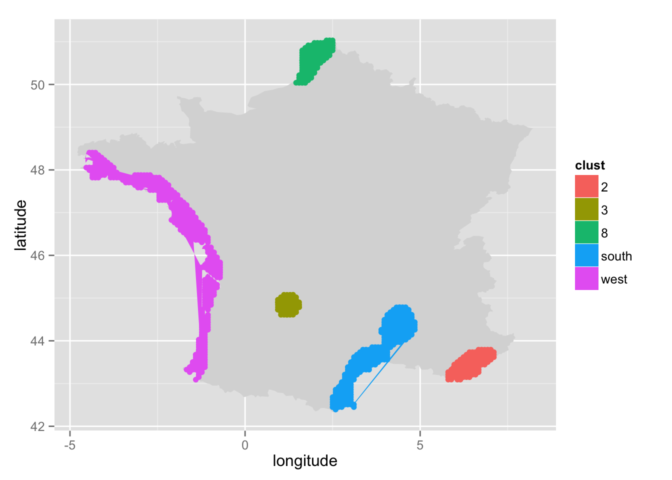
First, let's try to create 9 clusters:
pre_cut <- pre_cut_f(x = smoothed_camping,
                     threshold = 0.037,
                     alpha = 0.05,
                     poly = france[, c("long", "lat")],
                     k = 9,
                     print = TRUE)
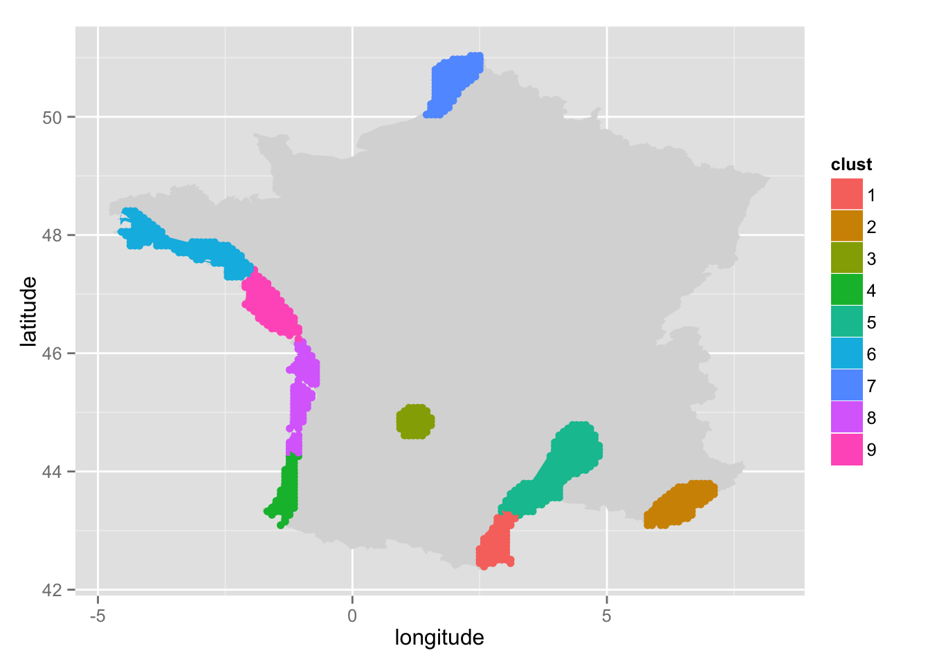
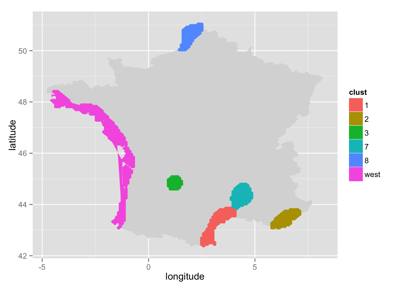
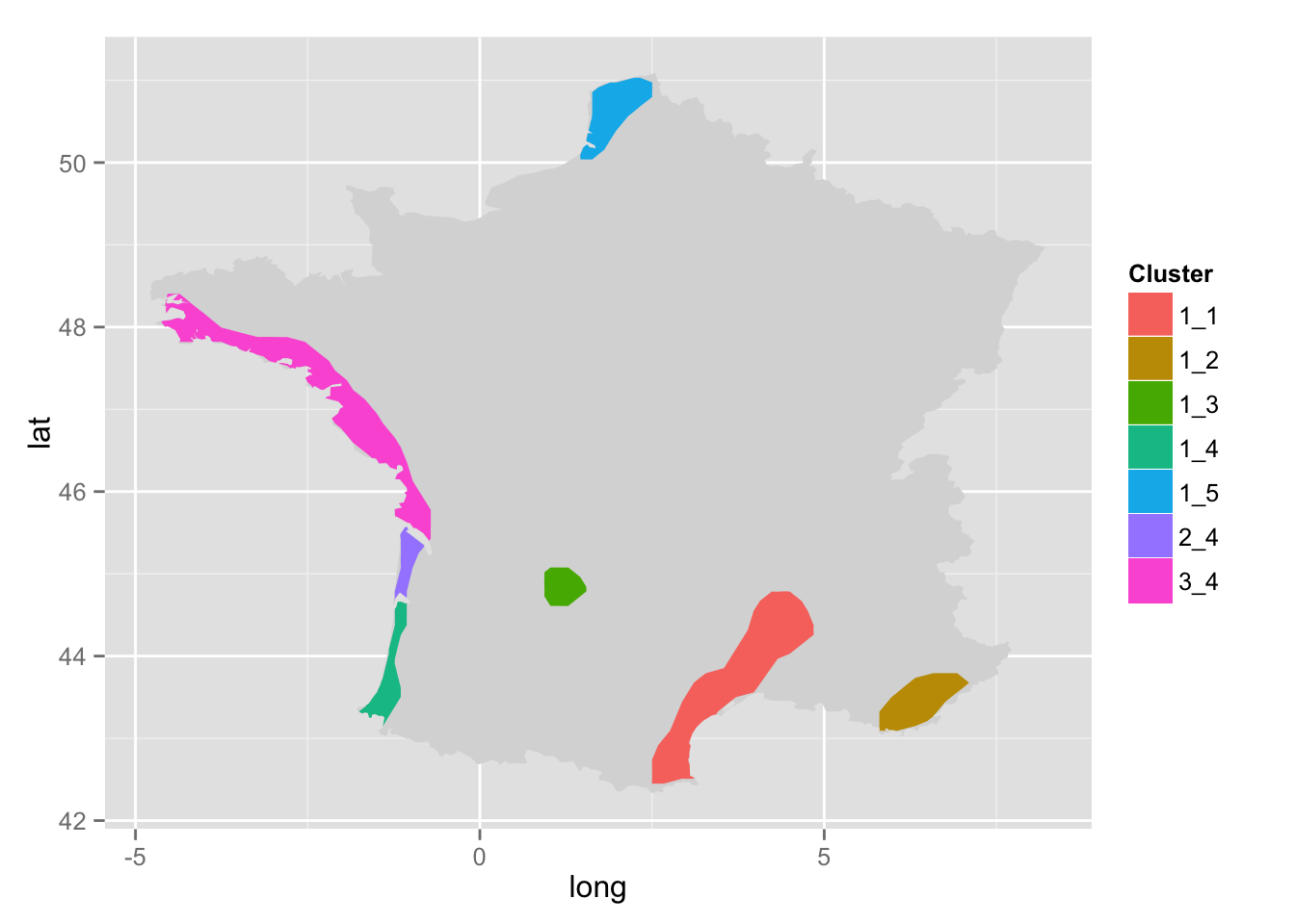
Then, we need to regroup the four polygons on the West. So we indicate that we want to regroup four polygons (n = 4). The name of the cluster will be "west" (group_name = "west"). We just need to click inside each polygon.
pre_cut <- regroup(pre_cut = pre_cut, poly = france[, c("long", "lat")],
                   n = 4, group_name = "west")
Then, let's do the same for the two polygons on the South:
pre_cut <- regroup(pre_cut = pre_cut, poly = france[, c("long", "lat")],
                   n = 2, group_name = "south")
We rely on gglocator() (package ggmap), so, if we need to print the map again, just before calling pre_cut(). It is important to use this function: print_map_help(), because we must provide a mapping parameter to ggplot(). Otherwise, gglocator() will fail.
# print_map_help(pre_cut, poly = france[, c("long", "lat")])
Once we're done, we simply call hull_polygons(), to get the coordinates!
hulls <- hull_polygons(pre_cut, france[,c("long", "lat")])
Result can be displayed on a map:
ggplot() + geom_polygon(data = france, aes(x = long, y = lat, group = group), fill = "grey85") +
  geom_polygon(data = hulls, aes(x = long, y = lat, group = group, fill = factor(group))) +
  scale_fill_discrete("Cluster")
Example 2: car accidents
First let us load the data. Once again, more details are given at https://github.com/ripleyCorr/Kernel_density_ripley/blob/master/README.md.
# Data can be obtained here: https://github.com/ripleyCorr/Kernel_density_ripley
load("../data/car_accidents/acci.RData")
load("../data/car_accidents/accidents.RData")
Let's try seven groups:
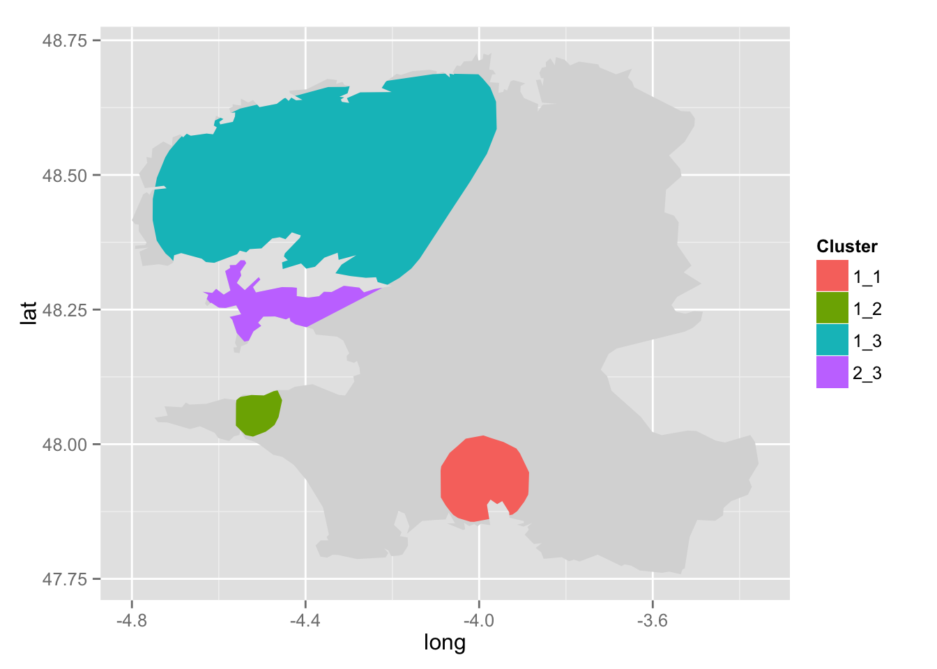
pre_cut <- pre_cut_f(x = accidents$finistere$smoothed,
                     threshold = 1.428,
                     alpha = 0.05,
                     poly = acci$finistere$polygon,
                     k = 7,
                     print = TRUE)
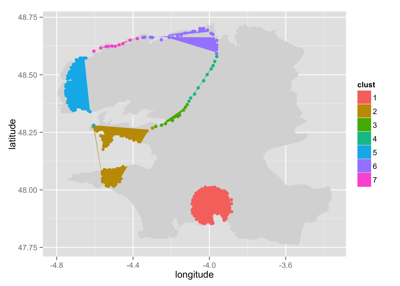
Regroup the groups in the North.
pre_cut <- regroup(pre_cut = pre_cut, poly = acci$finistere$polygon,
                   n = 5, group_name = "north")
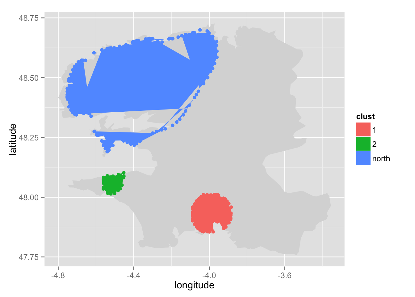
Then extract coordinates for each polygon.
hulls <- hull_polygons(pre_cut, acci$finistere$polygon, alpha = .9)
Anf finally, plot the result.
ggplot() + geom_polygon(data = acci$finistere$polygon, aes(x = long, y = lat), fill = "grey85") +
  geom_polygon(data = hulls, aes(x = long, y = lat, group = group, fill = factor(group))) +
  scale_fill_discrete("Cluster")